
In the previous blog post, we have shown how to leverage Debezium to train neural-network model with the existing data from the database and use this pre-trained model to classify images newly stored into the database. In this blog post, we will move it one step further - we will use Debezium to create multiple data streams from the database and use one of the streams for continuous learning and to improve our model, and the second one for making predictions on the data. When the model is constantly improved or adjusted to recent data samples, this approach is known as online machine learning. Online learning is only suitable for some use cases, and implementing an online variant of a given algorithm may be challenging or even impossible. However, in situations where online learning is possible, it becomes a very powerful tool as it allows one to react to the changes in the data in real-time and avoids the need to re-train and re-deploy new models, thus saving the hardware and operational costs. As the streams of data become more and more common, e.g. with the advent of IoT, we can expect online learning to become more and more popular. It’s usually a perfect fit for analyzing streaming data in use cases where it’s possible.
As mentioned in the previous blog, our goal here is not to build the best possible model for a given use case but to investigate how we can build a complete pipeline from inserting the data into the database through delivering it to the model and using it for model training and predictions. To keep things simple, we will use another well-known data sample often used in ML tutorials. We will explore how to classify various species of the Iris flower using an online variant of k-mean clustering algorithm. We use Apache Flink and Apache Spark to process the data streams. Both these frameworks are very popular data processing frameworks and include a machine learning library, which, besides others, implements online k-means algorithms. Thus, we can focus on building a complete pipeline for delivering the data from the database into a given model, processing it in real time, and not having to deal with the algorithm’s implementation details.
All the code mentioned later in this blog post is available as a Debezium example in Debezium example repository, with all other useful stuff, like Docker composes and step-by-step instructions in the README file.
Data set preparation
We will use Iris flower data set. Our goal is to determine the Iris species based on a couple of measurements of the Iris flower: its sepal length, sepal width, petal length, and petal width.
The data set can be downloaded from various sources. We can take advantage of the fact that it’s available already pre-processed in e.g. scikit-learn toolkit and use it from there. Each sample row contains a data point (sepal length, sepal width, petal length, and petal width) and a label. Label is number 0, 1, or 2, where 0 stands for Iris setosa, 1 stands for Iris versicolor, and 2 for Iris virginica. The data set is small - containing only 150 data points.
As we load the data into the database, we will first prepare SQL files, which we will later pass to the database. We need to divide the original data sample into three sub-samples - two for training and one for testing. The initial training will use the first training data sample. This data sample is intentionally small to not generate good predictions when we test the model for the first time so that we can see how the model’s prediction will increase in real-time when we feed it with more data.
You can use the following Python script from the accompanying demo repository for generating all three SQL files.
$ ./iris2sql.pyThe postgres directory contains the files used for this demo. train1.sql will be loaded automatically into the Postgres database upon its start. test.sql and train2.sql will be loaded manually into the database later.
Classification with Apache Flink
First, let’s look at how to do online Iris flower classification and learning in Apache Flink. The following figure depicts the high-level schema for the entire pipeline.
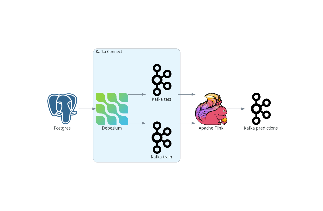
We will use Postgres as our source database. Debezium, deployed as a Kafka Connect source connector, tracks the changes in the database and creates the streams of data sent to Kafka from newly inserted data. Kafka sends these streams to Apache Flink, which employs the streaming k-means algorithm for model fitting and data classification. The predictions of the model for test data streams are produced as another stream and sent back to Kafka.
| You can also ingest database changes directly into the Flink without using Kafka. Ververika’s implementation of CDC source connectors embeds the Debezium directly into the Flink. See Flink CDC connectors documentation for more details. |
Our database contains two tables. The first stores our training data, while the second stores the test data. Therefore, there are two data streams, each corresponding to one table - one data stream for learning and one with data points that need to be classified. In real applications, you can use only one table or, on the contrary, many more tables. You can even deploy more Debezium connectors and thus combine data from several databases.
Using Debezium and Kafka as a source data stream
Apache Flink has excellent integration with Kafka. We can pass the Debezium records as e.g. JSON records. For creating Flink tables, it even has support for Debezium’s record format, but for streams, we need to extract part of the Debezium message, which contains the newly stored row of the table. However, this is very easy as Debezium provides SMT, extract new record state SMT, which does precisely this. The complete Debezium configuration can look like this:
{
    "name": "iris-connector-flink",
    "config": {
        "connector.class": "io.debezium.connector.postgresql.PostgresConnector",
        "tasks.max": "1",
        "database.hostname": "postgres",
        "database.port": "5432",
        "database.user": "postgres",
        "database.password": "postgres",
        "database.dbname" : "postgres",
        "topic.prefix": "flink",
        "table.include.list": "public.iris_.*",
        "key.converter": "org.apache.kafka.connect.json.JsonConverter",
        "value.converter": "org.apache.kafka.connect.json.JsonConverter",
        "transforms": "unwrap",
        "transforms.unwrap.type": "io.debezium.transforms.ExtractNewRecordState"
    }
}
The configuration captures all tables in the public schema with tables that begin with the iris_ prefix. Since we are storing training and test data in two tables, two Kafka topics named flink.public.iris_train and flink.public.iris_test are created, respectively. Flink’s DataStreamSource represents the incoming stream of data. As we encode the records as a JSON, it will be a stream of JSON ObjectNode objects. Constructing the source stream is very straightforward:
KafkaSource<ObjectNode> train = KafkaSource.<ObjectNode>builder()
    .setBootstrapServers("kafka:9092")
    .setTopics("flink.public.iris_train")
    .setClientIdPrefix("train")
    .setGroupId("dbz")
    .setStartingOffsets(OffsetsInitializer.earliest())
    .setDeserializer(KafkaRecordDeserializationSchema.of(new JSONKeyValueDeserializationSchema(false)))
    .build();
DataStreamSource<ObjectNode> trainStream = env.fromSource(train, WatermarkStrategy.noWatermarks(), "Debezium train");
Flink operates primarily on the Table abstraction object. Also, ML models accept only tables as input, and predictions are produced as tables too. Therefore, we must first convert our input stream into a Table object. We will start by transforming our input data stream into a stream of table rows. We need to define a map function that would return a Row object with a vector containing one data point. As the k-means algorithm belongs to unsupervised learning algorithms, i.e. the model doesn’t need corresponding "right answers" for the data points, we can skip the label field from the vector:
private static class RecordMapper implements MapFunction<ObjectNode, Row> {
    @Override
    public Row map(ObjectNode node) {
        JsonNode payload = node.get("value").get("payload");
        StringBuffer sb = new StringBuffer();
        return Row.of(Vectors.dense(
                        payload.get("sepal_length").asDouble(),
                        payload.get("sepal_width").asDouble(),
                        payload.get("petal_length").asDouble(),
                        payload.get("petal_width").asDouble()));
    }
}
Various parts of the internal Flink pipeline can run on different worker nodes, and therefore, we also need to provide type information about the table. With that, we are ready to create the table object:
StreamTableEnvironment tEnv = StreamTableEnvironment.create(env);
TypeInformation<?>[] types = {DenseVectorTypeInfo.INSTANCE};
String names[] = {"features"};
RowTypeInfo typeInfo = new RowTypeInfo(types, names);

DataStream<Row> inputStream = trainStream.map(new RecordMapper()).returns(typeInfo);
Table trainTable = tEnv.fromDataStream(inputStream).as("features");
Building Flink stream k-means
Once we have a Table object, we can pass it to our model. So let’s create one and pass a train stream to it for continuous model training:
OnlineKMeans onlineKMeans = new OnlineKMeans()
    .setFeaturesCol("features")
    .setPredictionCol("prediction")
    .setInitialModelData(tEnv.fromDataStream(env.fromElements(1).map(new IrisInitCentroids())))
    .setK(3);
OnlineKMeansModel model = onlineKMeans.fit(trainTable);
To make things more straightforward, we directly set the number of desired clusters to 3 instead of finding the optimal number of clusters by digging into the data (using e.g. elbow method). We also set some initial values for the centers of the clusters instead of using random numbers (Flink provides a convenient method for it - KMeansModelData.generateRandomModelData() if you want to try with random centers).
To obtain the predictions for our test data, we again need to convert our test stream into a table. The model transforms the table with test data into a table with predictions. Finally, convert the prediction into a stream and persisted, e.g. in a Kafka topic:
DataStream<Row> testInputStream = testStream.map(new RecordMapper()).returns(typeInfo);
Table testTable = tEnv.fromDataStream(testInputStream).as("features");
Table outputTable = model.transform(testTable)[0];

DataStream<Row> resultStream = tEnv.toChangelogStream(outputTable);
resultStream.map(new ResultMapper()).sinkTo(kafkaSink);
Now, we are ready to build our application and almost ready to submit it to Flink for execution. Before we do, we need to create the required Kafka topics first. While the topics can be empty, Flink requires that they at least exist. As we include a small set of data in the Postgres training table when the database starts, Debezium will create a corresponding topic when registering the Debezium Postgres connector in Kafka Connect. Since the test data table does not yet exist, we need to create the topic in Kafka manually:
$ docker compose -f docker-compose-flink.yaml exec kafka /kafka/bin/kafka-topics.sh --create --bootstrap-server kafka:9092 --replication-factor 1 --partitions 1 --topic flink.public.iris_testNow, we are ready to submit our application to Flink. For the complete code, please see the corresponding source code in Debezium example repository
| If you don’t use Docker compose provided as part of the source code for this demo, please include Flink ML library in the Flink |
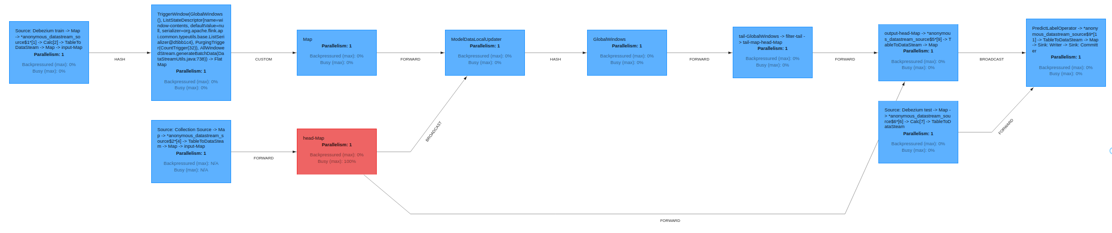
Flink provides a friendly UI, which is available on http://localhost:8081/. There, you can check, besides other things, the status of your jobs and also, e.g. job execution plan in an excellent graphical representation:
Evaluating the model
From the user’s point of view, all the interactions with our model occur by inserting new records into the database or reading Kafka topics with predictions. As we already created a very small initial training data sample in the database when it started, we can directly check our model predictions by inserting our test data sample into the database:
$ psql -h localhost -U postgres -f postgres/iris_test.sqlThe insert results in an immediate data stream of test data in Kafka, passing it into the model and sending the prediction back to the iris_predictions Kafka topic. The predictions are not accurate when training the model on a very small data set with just two clusters. The following shows our initial predictions:
[5.4, 3.7, 1.5, 0.2] is classified as 0
[4.8, 3.4, 1.6, 0.2] is classified as 0
[7.6, 3.0, 6.6, 2.1] is classified as 2
[6.4, 2.8, 5.6, 2.2] is classified as 2
[6.0, 2.7, 5.1, 1.6] is classified as 2
[5.4, 3.0, 4.5, 1.5] is classified as 2
[6.7, 3.1, 4.7, 1.5] is classified as 2
[5.5, 2.4, 3.8, 1.1] is classified as 2
[6.1, 2.8, 4.7, 1.2] is classified as 2
[4.3, 3.0, 1.1, 0.1] is classified as 0
[5.8, 2.7, 3.9, 1.2] is classified as 2
In our case, the correct answer should be:
[5.4, 3.7, 1.5, 0.2] is 0
[4.8, 3.4, 1.6, 0.2] is 0
[7.6, 3.0, 6.6, 2.1] is 2
[6.4, 2.8, 5.6, 2.2] is 2
[6.0, 2.7, 5.1, 1.6] is 1
[5.4, 3.0, 4.5, 1.5] is 1
[6.7, 3.1, 4.7, 1.5] is 1
[5.5, 2.4, 3.8, 1.1] is 1
[6.1, 2.8, 4.7, 1.2] is 1
[4.3, 3.0, 1.1, 0.1] is 0
[5.8, 2.7, 3.9, 1.2] is 1
When comparing the result, we only have 5 of 11 data points correctly classified due to the initial sample training data size. On the other hand, as we didn’t start with completely random clusters, our predictions are also not completely wrong.
Let’s see how things change when we supply more training data into the model:
$ psql -h localhost -U postgres -f postgres/iris_train2.sqlTo see the updated predictions, we insert the same test data sample again into the database:
$ psql -h localhost -U postgres -f postgres/iris_test.sqlThe following predictions are much better since we have all three categories present. We have also correctly classified 7 out of the 11 data points.
[5.4, 3.7, 1.5, 0.2] is classified as 0
[4.8, 3.4, 1.6, 0.2] is classified as 0
[7.6, 3.0, 6.6, 2.1] is classified as 2
[6.4, 2.8, 5.6, 2.2] is classified as 2
[6.0, 2.7, 5.1, 1.6] is classified as 2
[5.4, 3.0, 4.5, 1.5] is classified as 2
[6.7, 3.1, 4.7, 1.5] is classified as 2
[5.5, 2.4, 3.8, 1.1] is classified as 1
[6.1, 2.8, 4.7, 1.2] is classified as 2
[4.3, 3.0, 1.1, 0.1] is classified as 0
[5.8, 2.7, 3.9, 1.2] is classified as 1
As the whole data sample is pretty small, for further model training we can re-use our second train data sample:
$ psql -h localhost -U postgres -f postgres/iris_train2.sql
$ psql -h localhost -U postgres -f postgres/iris_test.sql
This results in the following prediction.
[5.4, 3.7, 1.5, 0.2] is classified as 0
[4.8, 3.4, 1.6, 0.2] is classified as 0
[7.6, 3.0, 6.6, 2.1] is classified as 2
[6.4, 2.8, 5.6, 2.2] is classified as 2
[6.0, 2.7, 5.1, 1.6] is classified as 2
[5.4, 3.0, 4.5, 1.5] is classified as 1
[6.7, 3.1, 4.7, 1.5] is classified as 2
[5.5, 2.4, 3.8, 1.1] is classified as 1
[6.1, 2.8, 4.7, 1.2] is classified as 1
[4.3, 3.0, 1.1, 0.1] is classified as 0
[5.8, 2.7, 3.9, 1.2] is classified as 1
We now find we have 9 out of 11 data points correctly classified. While this is still not an excellent result, we expect only partially accurate results as this is simply a prediction. The primary motivation here is to show the whole pipeline and demonstrate that the model improves the predictions without re-training and re-deploying the model when adding new data.
Classification with Apache Spark
From the user’s point of view, Apache Spark is very similar to Flink, and the implementation would be quite similar. This chapter is briefer to make this blog post more digestible.
Spark has two streaming models: the older DStreams, which is now in legacy state, and the more recent and recommended structured streaming. However, as the streaming k-means algorithm contained in the Spark ML library works only with the DStreams, for simplicity, DStreams are used in this example. A better approach would be to use structured streaming and implement the streaming k-means ourselves. This is, however, outside this blog post’s scope and main goal.
Spark supports streaming from Kafka using DStreams. However, writing DStreams back to Kafka is not supported, although it is possible but isn’t straightforward.
| Structured streaming supports both directions, reading and writing to Kafka, very easily. |
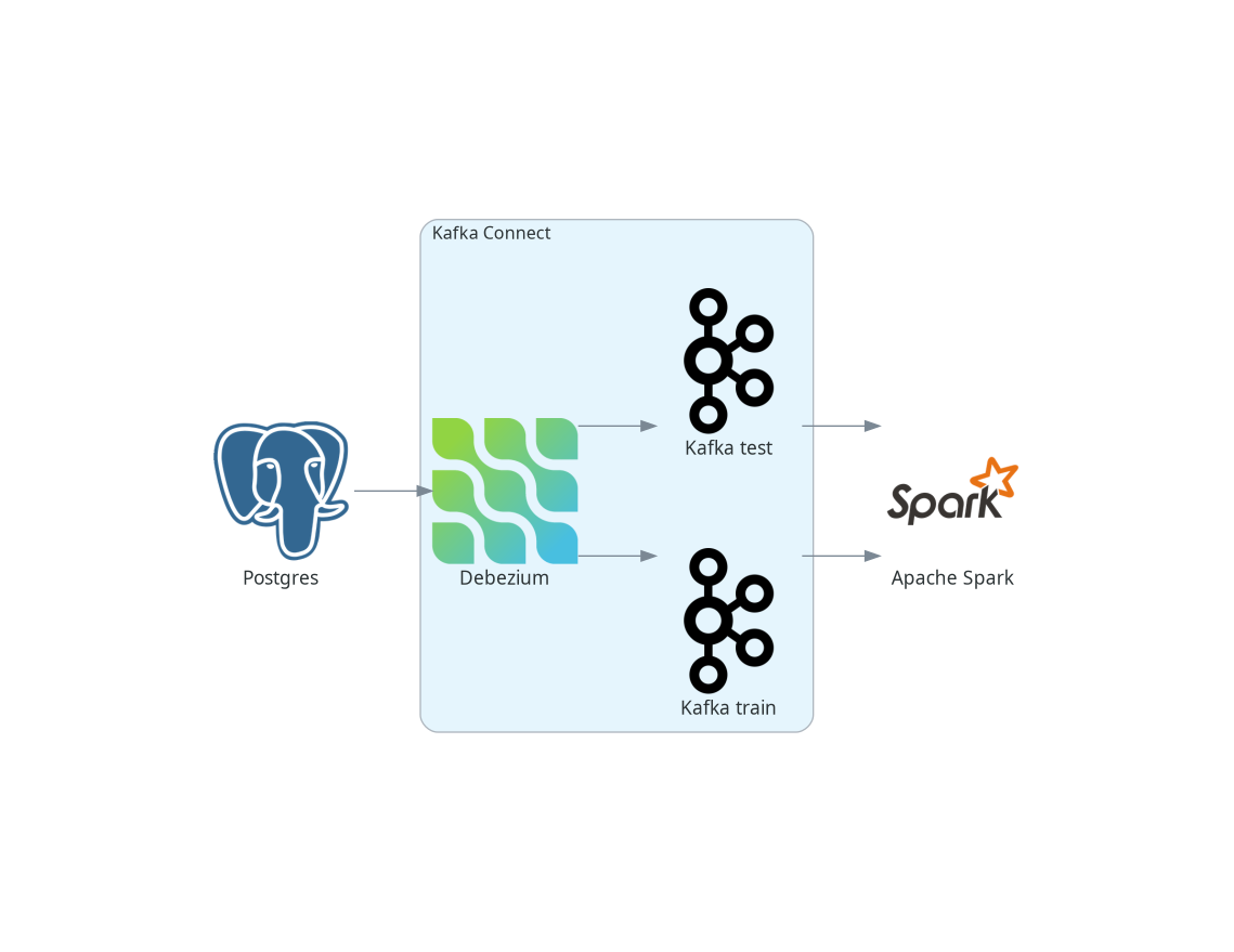
Again, for the sake of simplicity, we skip the final part and will write the predictions only to the console instead of writing them back to Kafka. The big picture of our pipelines thus looks like this:
Defining the data streams
Similarly to Flink, creating Spark streams from Kafka streams is straightforward, and most of the parameters are self-explanatory:
Set<String> trainTopic = new HashSet<>(Arrays.asList("spark.public.iris_train"));
Set<String> testTopic = new HashSet<>(Arrays.asList("spark.public.iris_test"));
Map<String, Object> kafkaParams = new HashMap<>();
kafkaParams.put(ConsumerConfig.BOOTSTRAP_SERVERS_CONFIG, "kafka:9092");
kafkaParams.put(ConsumerConfig.GROUP_ID_CONFIG, "dbz");
kafkaParams.put(ConsumerConfig.AUTO_OFFSET_RESET_CONFIG, "earliest");
kafkaParams.put(ConsumerConfig.KEY_DESERIALIZER_CLASS_CONFIG, StringDeserializer.class);
kafkaParams.put(ConsumerConfig.VALUE_DESERIALIZER_CLASS_CONFIG, StringDeserializer.class);

JavaInputDStream<ConsumerRecord<String, String>> trainStream = KafkaUtils.createDirectStream(
        jssc,
        LocationStrategies.PreferConsistent(),
        ConsumerStrategies.Subscribe(trainTopic, kafkaParams));
JavaDStream<LabeledPoint> train = trainStream.map(ConsumerRecord::value)
        .map(SparkKafkaStreamingKmeans::toLabeledPointString)
        .map(LabeledPoint::parse);
On the last line, we transform the Kafka stream to a labeled point stream, which the Spark ML library uses for working with its ML models. Labeled points are expected as the strings formatted as data point labels separated by the comma from space-separated data point values. So the map function looks like this:
private static String toLabeledPointString(String json) throws ParseException {
    JSONParser jsonParser = new JSONParser();
    JSONObject o = (JSONObject)jsonParser.parse(json);
    return String.format("%s, %s %s %s %s",
            o.get("iris_class"),
            o.get("sepal_length"),
            o.get("sepal_width"),
            o.get("petal_length"),
            o.get("petal_width"));
}
It still applies that k-means is an unsupervised algorithm and doesn’t use the data point labels. However, it’s convenient to pass them to LabeledPoint class as later on, we can show them together with model predictions.
We chain one more map function to parse the string and create a labeled data point from it. In this case, it’s a built-in function of Spark LabeledPoint.
Contrary to Flink, Spark doesn’t require Kafka topics to exist in advance, so when deploying the model, we don’t have to create the topics. We can let Debezium create them once the table with the test data is created and populated with the data.
Defining and evaluating the model
Defining the streaming k-means model is very similar to Flink:
StreamingKMeans model = new StreamingKMeans()
        .setK(3)
        .setInitialCenters(initCenters, weights);
model.trainOn(train.map(lp -> lp.getFeatures()));
Also, in this case, we directly set the number of clusters to 3 and provide the same initial central points to the clusters. We also only pass the data points for training, not the labels.
As mentioned above, we can use the labels to show them together with the predictions:
JavaPairDStream<Double, Vector> predict = test.mapToPair(lp -> new Tuple2<>(lp.label(), lp.features()));
model.predictOnValues(predict).print(11);
We print 11 stream elements to the console on the resulting stream with the predictions, as this is the size of our test sample. Like Flink, the results after initial training on a very small data sample could be better. The first number in the tuple is the data point label, while the second one is the corresponding prediction done by our model:
spark_1      | (0.0,0)
spark_1      | (0.0,0)
spark_1      | (2.0,2)
spark_1      | (2.0,2)
spark_1      | (1.0,0)
spark_1      | (1.0,0)
spark_1      | (1.0,2)
spark_1      | (1.0,0)
spark_1      | (1.0,0)
spark_1      | (0.0,0)
spark_1      | (1.0,0)
However, when we provide more training data, predictions are much better:
spark_1      | (0.0,0)
spark_1      | (0.0,0)
spark_1      | (2.0,2)
spark_1      | (2.0,2)
spark_1      | (1.0,1)
spark_1      | (1.0,1)
spark_1      | (1.0,2)
spark_1      | (1.0,0)
spark_1      | (1.0,1)
spark_1      | (0.0,0)
spark_1      | (1.0,0)
If we pass the second training data sample once again for the training, our model makes correct predictions for the whole test sample:
---
spark_1      | (0.0,0)
spark_1      | (0.0,0)
spark_1      | (2.0,2)
spark_1      | (2.0,2)
spark_1      | (1.0,1)
spark_1      | (1.0,1)
spark_1      | (1.0,1)
spark_1      | (1.0,1)
spark_1      | (1.0,1)
spark_1      | (0.0,0)
spark_1      | (1.0,1)
----| The prediction is a number of the cluster which k-means algorithm created and has no relation to labels in our data sample. That means that e.g. |
So, similar to Flink, we get better results as we pass more training data without the need to re-train and re-deploy the model. In this case, we get even better results than Flink’s model.
Conclusions
In this blog post, we continued exploring how Debezium can help make data ingestion into various ML frameworks seamless. We have shown how to pass the data from the database to Apache Flink and Apache Spark in real time as a stream of the data. The integration is easy to set up in both cases and works well. We demonstrated it in an example that allows us to use an online learning algorithm, namely the online k-means algorithm, to highlight the power of data streaming. Online machine learning allows us to make real-time predictions on the data stream and improve or adjust the model immediately as the new training data arrives. Model adjustment doesn’t require any model re-training on a separate compute cluster and re-deploying a new model, making ML-ops more straightforward and cost-effective.
As usual, we would appreciate any feedback on this blog post. Do you have any ideas on how Debezium or change data capture can be helpful in this area? What would be helpful to investigate, whether integration with another ML framework, integration with a specific ML feature store, etc.? In case you have any input any this regard, don’t hesitate to reach out to us on the Zulip chat, mailing list or you can transform your ideas directly into Jira feature requests.
About Debezium
Debezium is an open source distributed platform that turns your existing databases into event streams, so applications can see and respond almost instantly to each committed row-level change in the databases. Debezium is built on top of Kafka and provides Kafka Connect compatible connectors that monitor specific database management systems. Debezium records the history of data changes in Kafka logs, so your application can be stopped and restarted at any time and can easily consume all of the events it missed while it was not running, ensuring that all events are processed correctly and completely. Debezium is open source under the Apache License, Version 2.0.
Get involved
We hope you find Debezium interesting and useful, and want to give it a try. Follow us on Twitter @debezium, chat with us on Zulip, or join our mailing list to talk with the community. All of the code is open source on GitHub, so build the code locally and help us improve ours existing connectors and add even more connectors. If you find problems or have ideas how we can improve Debezium, please let us know or log an issue.