
With the recent success of ChatGPT, we can observe another wave of interest in the AI field and machine learning in general. The previous wave of interest in this field was, at least to a certain extent, caused by the fact that excellent ML frameworks like TensorFlow, PyTorch or general data processing frameworks like Spark became available and made the writing of ML models much more straightforward. Since that time, these frameworks have matured, and writing models are even more accessible, as you will see later in this blog. However, data set preparation and gathering data from various sources can sometimes take time and effort. Creating a complete pipeline that would pull existing or newly created data, adjust it, and ingest it into selected ML libraries can be challenging. Let’s investigate if Debezium can help with this task and explore how we can leverage Debezium’s capabilities to make it easier.
Change data capture and Debezium in ML pipelines
Change data capture (CDC) can be a compelling concept in machine learning, especially in online machine learning. However, using pre-trained models, CDC can also be an essential part of the pipeline. We can use CDC to deliver new data immediately into a pre-trained model, which can evaluate it, and other parts of the pipeline can take any action based on the model output in real-time.
Besides these use cases, Debezium is a perfect fit for any pipeline, including loading data from databases. Debezium can capture existing data as well as stream any newly created data. Another vital feature of Debezium is support for single message transforms. We can adjust the data at the very beginning of the whole pipeline. When applying transformations or filters, we can restrict data transmission over the wire to only that is of interest, saving bandwidth and speed within the pipeline. Additionally, Debezium can deliver records to several message brokers, and more brokers are being added (several new ones are available in the recent 2.2.0 release). These continued improvements increase the opportunity to integrate Debezium with other toolchains or data pipelines. The possibilities are endless, and Debezium’s common connector framework could allow for CDC beyond just databases.
So, this is the theory. Now let’s explore how it works in reality. This blog post will look at how to stream data into TensorFlow. Based on the interest from the community, this may result in a series of blog posts where we explore possible integrations with other ML libraries and frameworks.
Debezium and TensorFlow integration
TensorFlow is one of the most popular machine learning frameworks. It provides a comprehensive platform for building, training, and deploying machine learning models across various applications.
To keep things simple, we will implement a model for recognizing handwritten digits, which is more or less the Hello World equivalent in the neural networks field. The ultimate goal of this demo is to use Debezium to load MNIST data samples from Postgres that are continuously stored, pass it to our model implemented in Tensorflow for training, and use this trained model for real-time classification of images
The diagram below depicts the complete pipeline:
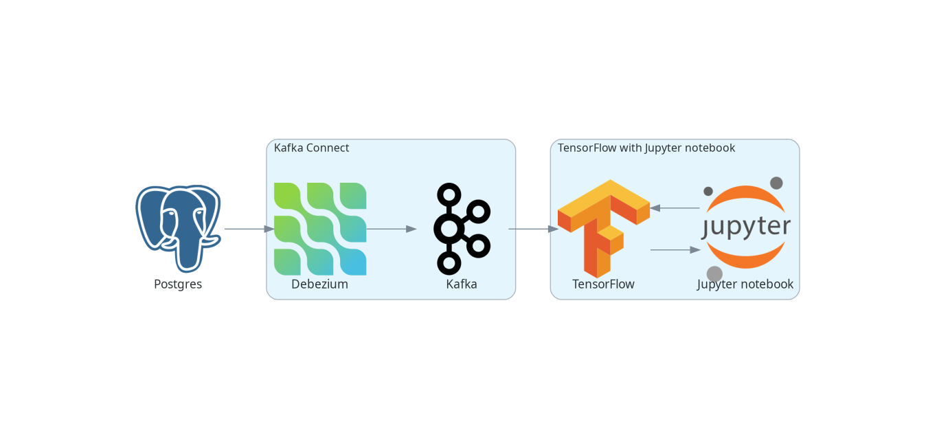
All the code mentioned later in this blog is available as a Debezium example in Debezium example repository.
The data sample
We will use MNIST data sample. The training sample contains 60,000 images with handwritten digits from 0 to 9 and the same amount of labels with corresponding digits. The test sample contains 1,000 images. The samples are available as gzip binaries. As we assume a use case where the data of interest are in the database, we need to load the data into the database first.
We need to generate two SQL files, one for the train data set, mnist_train.sql, and one for a test data sample, mnist_test.sql. Each file would contain SQL commands for creating a table with two columns: pixels column of type BYTEA, which would contain raw image bytes, and labels column of type SMALLINT, which would contain digit corresponding to the image in given table row. The rest of the file would contain commands for populating the table. Image bytes can be decoded as a HEX string.
As we will show how to leverage Debezium for data streaming later in this post, we will initially load the training data set into the database. The SQL file with training data will be used directly by the Postgres container - when it starts, it will load this data into the training table. We will use the test data SQL file later. However, the preparation of the data is the same for training as well as test samples, and we can prepare both of them in one go.
To prepare these SQL files, you can use mnist2sql.py script from Debezium tensorflow-mnist example:
$ ./mnist2sql.py --downloadThe script assumes MNIST data sets are available in the postgres directory. When using the --download parameter, the script first downloads MNIST data samples into the postgres directory. The postgres directory will contain the resulting SQL files.
Loading streamed data into Tensorflow
The most common Debezium usage is the streaming of records to Kafka. TensorFlow provides TensorFlow I/O module for loading data from various sources. Besides other sources, it also allows loading the data from Kafka. There are several ways to do it. IODataset.from_kafka() method loads only existing data from specified Kafka topics. Two experimental classes support streaming data, KafkaBatchIODataset and KafkaGroupIODataset. Both are very similar and allow them to work with streaming data, i.e., they not only read the existing data from a Kafka topic but also wait for new data and eventually pass new records into the TensorFlow. Streaming concludes when there are no new events within a specified time frame.
In all cases, a Dataset represents all loaded records in Tensorflow. This Tensorflow data structure provides convenience for building data pipelines, which may include further data transformations or preprocessing.
This sounds great. However, the most significant caveat is the representation of records within the Dataset. These Kafka loaders completely ignore the schema of the records provided by Kafka, meaning that keys and values are raw bytes of data. Additionally, the ingestion pipeline complicates the process by converting these into strings (i.e., toString() on the object called). So if you pass, e.g., raw image bytes via Kafka, using Kafka BYTES_SCHEMA, it would result in something like this:
<tf.Tensor: shape=(64,), dtype=string, numpy=
 array([b'[B@418b353d', b'[B@6aa28a4c', b'[B@b626485', b'[B@6d7491cd',
        b'[B@13fa86c5', b'[B@7c3bc352', b'[B@64e5d61c', b'[B@2dd6d9b4',
        b'[B@6addae65', b'[B@48ded13f', b'[B@2c1bb0e', b'[B@19c1d99b',
        b'[B@1ee8f240', b'[B@20019f8b', b'[B@2f17494e', b'[B@380d4036',
        b'[B@61aecf85', b'[B@4d7fe9fc', b'[B@58b79424', b'[B@ae963f4',
        b'[B@1dac57cb', b'[B@2fae7d8b', b'[B@4b5ccaee', b'[B@aebf6b2',
        b'[B@7506ea2b', b'[B@29989325', b'[B@43e2742', b'[B@51350f11',
        b'[B@13a0f0ae', b'[B@7e4c4844', b'[B@b3d64f8', b'[B@7209bf09',
        b'[B@66380466', b'[B@7aaa7e8d', b'[B@1ad0cf84', b'[B@259eca20',
        b'[B@3a3f1c1', b'[B@36e4ff1f', b'[B@6578fc29', b'[B@79c924be',
        b'[B@765b7f70', b'[B@67567aa3', b'[B@456d4bd4', b'[B@75317b13',
        b'[B@58bc3a3a', b'[B@c6bc0ec', b'[B@2377095e', b'[B@5de017c0',
        b'[B@64b48bac', b'[B@360a5b76', b'[B@2d2c9910', b'[B@70afd562',
        b'[B@3006c930', b'[B@54b3e5ad', b'[B@1d1e0232', b'[B@1394d036',
        b'[B@155dd43d', b'[B@5e88d5b6', b'[B@33ea53c7', b'[B@64a30ec',
        b'[B@7dcdf024', b'[B@6570bf4e', b'[B@4e5bc4c', b'[B@537f216c'],
       dtype=object)>,
Instead of getting a batch of raw image bytes which you can further transform in TensorFlow, you get only string representation of Java byte arrays, which is not very useful.
The most straightforward solution would be to convert the raw image bytes into numbers before sending them to Kafka to mitigate the problem. As TensorFlow provides methods for parsing CSV input, we can convert each image into one CSV line of numbers. Since Tensorflow primarily works with numbers, we would be required to convert the images to numbers regardless. We can pass the number on the image as a message key. Now, a single message transform supported by Debezium comes in handy. The transformation can look like this:
    @Override
    public R apply(R r) {
        final Struct value = (Struct) r.value();
        String key = value.getInt16(labelFieldName).toString();

        StringBuilder builder = new StringBuilder();
        for (byte pixel : value.getBytes(pixlesFieldName)) {
            builder.append(pixel & 0xFF).append(",");
        }
        if (builder.length() > 0) {
            builder.deleteCharAt(builder.length() - 1);
        }
        String newValue = builder.toString();

        return r.newRecord(r.topic(), r.kafkaPartition(), Schema.STRING_SCHEMA, key, Schema.STRING_SCHEMA, newValue, r.timestamp());
    }
On the TensorFlow side, we must convert bytes obtained from Kafka messages into numbers. The following illustrates a map function to handle this easily:
def decode_kafka_record(record):
    img_int = tf.io.decode_csv(record.message, [[0.0] for i in range(NUM_COLUMNS)])
    img_norm = tf.cast(img_int, tf.float32) / 255.
    label_int = tf.strings.to_number(record.key, out_type=tf.dtypes.int32)
    return (img_norm, label_int)
Here we parse CSV lines, potentially provided as the raw bytes, and immediately scale the numbers within the <0, 1> interval, which is convenient for training our model later. Loading the data and creating data batches is very straightforward:
train_ds = tfio.IODataset.from_kafka(KAFKA_TRAIN_TOPIC, partition=0, offset=0, servers=KAFKA_SERVERS)
train_ds = train_ds.map(decode_kafka_record)
train_ds = train_ds.batch(BATCH_SIZE)
Here we use IODataset.from_kafka() for loading existing data from the Kafka topic, use our map function to convert bytes into numbers, and scale the numbers. As a last step, we create batches from the data set for more efficient processing. Parameters of tfio.IODataset.from_kafka() are self-explanatory and probably don’t need further comments.
As a result, we have a data set formed by two-dimensional tensors. The first dimension is a vector of floats representing the image, while the second dimension is a single number (scalar) describing the number on the picture. Once we have prepared our training data set, we can define our neural network model.
Defining the model
To keep things simple, as the main goal of this post is not to show the best handwritten digit classifier, but to show how to create the data pipeline, let’s use a very simple model:
model = tf.keras.models.Sequential([
    tf.keras.layers.Dense(128, activation='relu'),
    tf.keras.layers.Dense(10)
])
This model contains only two layers. Although this model is really simple, it still does a pretty good job in recognition of handwritten digits. Probably more interesting than the model itself is how easy it is to write a mode in TensorFlow (or actually Keras, but it’s now part of TensorFlow).
Similarly easy is to define model optimizer and the loss function:
model.compile(
    optimizer=tf.keras.optimizers.Adam(0.001),
    loss=tf.keras.losses.SparseCategoricalCrossentropy(from_logits=True),
    metrics=[tf.keras.metrics.SparseCategoricalAccuracy()],
)
It’s outside of this post’s scope to explain these functions, and you can check almost any machine learning online course or textbook on this topic for a detailed explanation.
Once we have our model ready, we can train it on the trained dataset prepared in the previous section:
model.fit(train_ds,epochs=MAX_EPOCHS)This step may take quite some time to finish. However, once finished, our model is ready to recognize handwritten digits!
Streaming the data into the model
Let’s see how good our model is in digit recognition. But as our primary goal here is to explore the means how to ingest data into TensorFlow, we will start model evaluation on an empty (or, more accurately, even non-existing) Kafka topic and see if we will be able to evaluate the data on the fly as they will pop-up first in the database and then in the corresponding Kafka topic. For this purpose, we can use one of the streaming classes mentioned above:
test_ds = tfio.experimental.streaming.KafkaGroupIODataset(
    topics=[KAFKA_TEST_TOPIC],
    group_id=KAFKA_CONSUMER_GROUP,
    servers=KAFKA_SERVERS,
    stream_timeout=9000,
    configuration=[
        "session.timeout.ms=10000",
        "max.poll.interval.ms=10000",
        "auto.offset.reset=earliest"
    ],
)
Again, arguments are mostly self-explanatory. Two things may need further explanation: stream_timeout and configuration parameters. stream_timeout determines the interval of inactivity (in milliseconds) after which the streaming would terminate. configuration is librdkafka configuration. It’s a configuration of the Kafka client; you should configure at least the session timeout (session.timeout.ms), and it’s poll interval (max.poll.interval.ms). The values of these parameters should be higher than the value of stream_timeout.
The dataset this loader provides is slightly different - instead of providing a single record containing the message and its key, we get the key and message already split. Therefore, we have to define a slightly modified map function with two arguments:
def decode_kafka_stream_record(message, key):
    img_int = tf.io.decode_csv(message, [[0.0] for i in range(NUM_COLUMNS)])
    img_norm = tf.cast(img_int, tf.float32) / 255.
    label_int = tf.strings.to_number(key, out_type=tf.dtypes.int32)
    return (img_norm, label_int)
With this function, we can adjust the dataset and create batches as before:
test_ds = test_ds.map(decode_kafka_stream_record)
test_ds = test_ds.batch(BATCH_SIZE)
and evaluate the model:
model.evaluate(test_ds)You can execute a cell with model evaluation in the Jupyter notebook. The execution will wait because there is no such topic in Kafka and no table with test data in the database. The streaming timeout is 9 seconds, so data must be provided within this time frame after launching the model evaluation. At the start of this demo, we created a SQL file in the postgres directory called mnist_test.sql, which can generate the test data we need:
$ export PGPASSWORD=postgres
$ psql -h localhost -U postgres -f postgres/mnist_test.sql
After a short while, you should see in the Jupyter notebook output that some data arrived into the model and, a few moments later final evaluation of the model.
To make the results closer to humans, let’s define an image manually and serve it to the model. We can also easily show the image in the Jypiter notebook. The function for plotting the images and providing model predictions as a plot title can look like this:
def plot_and_predict(pixels):
    test = tf.constant([pixels])
    tf.shape(test)
    test_norm = tf.cast(test, tf.float32) / 255.

    prediction = model.predict(test_norm)
    number = tf.nn.softmax(prediction).numpy().argmax()

    pixels_array = np.asarray(pixels)
    raw_img = np.split(pixels_array, 28)
    plt.imshow(raw_img)
    plt.title(number)
    plt.axis("off")
Probably the only cryptic line in this function is the one containing the softmax() function. This function converts the resulting vector into a vector of probabilities. Elements of this vector express the probability that the number on a given position is the one on the image. Therefore, the position with the highest probability is the model’s prediction, where argmax() is derived.
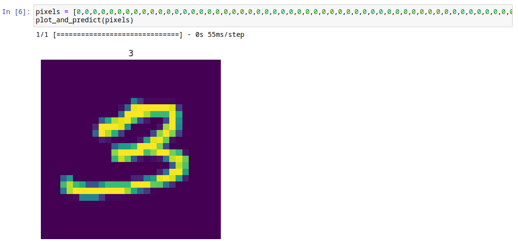
We can try it, e.g., for this image, which contains the handwritten number 3:
pixels = [0,0,0,0,0,0,0,0,0,0,0,0,0,0,0,0,0,0,0,0,0,0,0,0,0,0,0,0,0,0,0,0,0,0,0,0,0,0,0,0,0,0,0,0,0,0,0,0,0,0,0,0,0,0,0,0,0,0,0,0,0,0,0,0,0,0,0,0,0,0,0,0,0,0,0,0,0,0,0,0,0,0,0,0,0,0,0,0,0,0,0,0,0,0,0,0,0,0,0,0,0,0,0,0,0,0,0,0,0,0,0,0,0,0,0,0,0,0,0,0,0,0,0,0,0,0,0,0,0,0,0,0,0,0,0,0,0,0,0,0,0,0,0,0,0,0,0,0,0,0,0,0,0,0,0,0,0,0,0,0,0,0,0,0,0,0,0,0,0,0,0,0,0,0,0,0,0,0,0,0,0,0,108,43,6,6,6,6,5,0,0,0,0,0,0,0,0,0,0,0,0,0,0,0,0,0,0,0,10,84,248,254,254,254,254,254,241,45,0,0,0,0,0,0,0,0,0,0,0,0,0,0,0,0,0,0,90,254,254,254,223,173,173,173,253,156,0,0,0,0,0,0,0,0,0,0,0,0,0,0,1,79,157,228,245,251,188,63,17,0,0,54,252,132,0,0,0,0,0,0,0,0,0,0,0,0,0,0,32,254,254,254,244,131,0,0,0,0,13,220,254,122,0,0,0,0,0,0,0,0,0,0,0,0,0,0,83,254,225,160,47,0,0,0,0,59,211,254,206,50,0,0,0,0,0,0,0,0,0,0,0,0,0,0,1,21,14,0,0,0,2,17,146,245,250,194,12,0,0,0,0,0,0,0,0,0,0,0,0,0,0,0,0,0,0,81,140,140,171,254,254,254,203,55,1,0,0,0,0,0,0,0,0,0,0,0,0,0,0,0,0,0,0,211,254,254,254,254,179,211,254,254,202,171,14,0,0,0,0,0,0,0,0,0,0,0,0,0,0,0,0,167,233,193,69,16,3,9,16,107,231,248,195,0,0,0,0,0,0,0,0,0,0,0,0,0,0,0,0,0,0,0,0,0,0,0,0,0,73,229,182,0,0,0,0,0,0,0,0,0,0,0,0,0,0,0,0,0,0,0,0,0,0,0,26,99,252,254,146,0,0,0,0,0,0,0,0,79,142,0,0,0,0,0,0,0,0,0,26,28,116,147,247,254,239,150,22,0,0,0,0,0,0,0,0,175,230,174,155,66,66,132,174,174,174,174,250,255,254,192,189,99,36,0,0,0,0,0,0,0,0,0,0,106,226,254,254,254,254,254,254,254,254,217,151,80,43,2,0,0,0,0,0,0,0,0,0,0,0,0,0,0,4,7,114,114,114,46,5,5,5,3,0,0,0,0,0,0,0,0,0,0,0,0,0,0,0,0,0,0,0,0,0,0,0,0,0,0,0,0,0,0,0,0,0,0,0,0,0,0,0,0,0,0,0,0,0,0,0,0,0,0,0,0,0,0,0,0,0,0,0,0,0,0,0,0,0,0,0,0,0,0,0,0,0,0,0,0,0,0,0,0,0,0,0,0,0,0,0,0,0,0,0,0,0,0,0,0,0,0,0,0,0,0,0,0,0,0,0,0,0,0,0,0,0,0,0,0,0,0,0,0,0,0,0,0,0,0,0,0,0,0,0,0,0,0,0,0,0,0,0,0,0,0,0,0,0,0,0,0,0,0,0,0,0,0,0,0,0,0,0,0,0,0,0,0,0,0,0,0,0,0,0,0,0,0,0,0,0,0,0,0,0,0]
plot_and_predict(pixels)
The result would be as follows:
You can do the same by reading from a Kafka stream, and we can reuse existing topics for this purpose. As we already read all records from the test stream, we need to change the Kafka consumer group if we want to reread it using streaming KafkaGroupIODataset:
manual_ds = tfio.experimental.streaming.KafkaGroupIODataset(
    topics=[KAFKA_TEST_TOPIC],
    group_id="mnistcg2",
    servers=KAFKA_SERVERS,
    stream_timeout=9000,
    configuration=[
        "session.timeout.ms=10000",
        "max.poll.interval.ms=10000",
        "auto.offset.reset=earliest"
    ],
)

manual_ds = manual_ds.map(decode_kafka_stream_record)
If you want to create a new stream and verify that our model can provide prediction as the new data arrives, you can easily do so:
$ head -5 mnist_test.sql | sed s/test/manual/ > mnist_manual.sql
$ psql -h localhost -U postgres -f postgres/mnist_manual.sql
In such case you don’t need to change Kafka consumer group, but you have to change the Kafka topic:
manual_ds = tfio.experimental.streaming.KafkaGroupIODataset(
topics=["tf.public.mnist_manual"],
group_id=KAFKA_CONSUMER_GROUP,
servers=KAFKA_SERVERS,
stream_timeout=9000,
configuration=[
"session.timeout.ms=10000",
"max.poll.interval.ms=10000",
"auto.offset.reset=earliest"
],
)
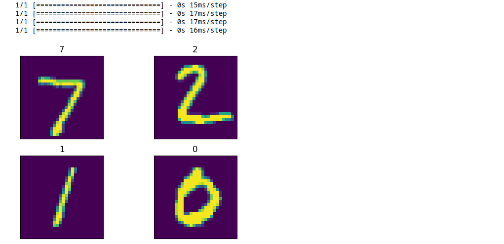
manual_ds = manual_ds.map(decode_kafka_stream_record)In either case, the result should look like this:
Conclusions
In this demo, we have shown how to load existing data from the database, transform it on the fly, ingest it into the TensorFlow model via Kafka, and use it for model training. Later on, we ingested newly created data into this pre-trained model using CDC and data streaming and obtained meaningful results. Debezium can provide valuable service not only for use cases like the one described in this post but can also play a key role in ingesting data to online machine learning pipelines.
While the whole pipeline is relatively easy to implement, some areas can be improved to improve the user experience and/or make the entire pipeline more smooth. As our (Debezium developers) background is not primarily in machine learning and data science, we would appreciate any input from the community on how Debezium can aid machine learning pipelines (or is already used, if there are any such cases) and where are the rooms for improvements. We would also appreciate any new ideas on how Debezium, or in general, change data capture, can be helpful in this area. These ideas further reveal Debezium’s potential to ingest data into machine learning pipelines and contribute to better user experience in the whole process. In case you have any input any this regard, don’t hesitate to reach out to us on the Zulip chat, mailing list or you can transform your ideas directly into Jira feature requests.
About Debezium
Debezium is an open source distributed platform that turns your existing databases into event streams, so applications can see and respond almost instantly to each committed row-level change in the databases. Debezium is built on top of Kafka and provides Kafka Connect compatible connectors that monitor specific database management systems. Debezium records the history of data changes in Kafka logs, so your application can be stopped and restarted at any time and can easily consume all of the events it missed while it was not running, ensuring that all events are processed correctly and completely. Debezium is open source under the Apache License, Version 2.0.
Get involved
We hope you find Debezium interesting and useful, and want to give it a try. Follow us on Twitter @debezium, chat with us on Zulip, or join our mailing list to talk with the community. All of the code is open source on GitHub, so build the code locally and help us improve ours existing connectors and add even more connectors. If you find problems or have ideas how we can improve Debezium, please let us know or log an issue.