
SQL Server offers change data capture (CDC) through change tables - a special set of system tables that record modifications in selected “ordinary” tables. If you want to monitor changes in real time, you query these change tables periodically. That’s exactly how Debezium works today: it polls SQL Server’s change tables at configured intervals and turns the results into a continuous stream of CDC records. This approach works fine, but could we do better?
Captured tables are filled by the SQL Server Agent, which reads the transaction log, extracts changes, and stores them in change tables. In theory, we could skip the middleman and parse the transaction log directly. That’s how tools like OpenLogReplicator handle CDC for Oracle databases. Let’s peek inside the SQL Server internals and explore little bit how it works and stores the records.
In this post, we’ll:
-
Prepare a local SQL Server instance for experimentation
-
Explore the internal structure of the SQL Server transaction log
-
Understand how the records are stored on the disk
Preparing SQL Server
We’ll set up SQL Server locally so we can poke around in its log files. You have two main options: Docker container or VM installation. Let’s take a look at both approaches.
Setting up SQL Server container
Using container is pretty straightforward, you just need to start it:
docker run -it --rm --name sqlserver \
  -e "ACCEPT_EULA=Y" \
  -e "MSSQL_SA_PASSWORD=Password!" \
  -p 1433:1433 mcr.microsoft.com/mssql/server:2022-latest
Once the container is running, you can connect directly from your host machine or attach to the container and use the built-in mssql-tools:
docker exec -it sqlserver /bin/bash
/opt/mssql-tools18/bin/sqlcmd -S localhost -U SA -P Password! -C -No
Setting up SQL Server in a VM
Follow the official guide for RHEL or Fedora. The steps for adding appropriate repo, installing and configuring the server are straightforward:
curl -o /etc/yum.repos.d/mssql-server.repo https://packages.microsoft.com/config/rhel/9/mssql-server-2022.repo
dnf install -y mssql-server
/opt/mssql/bin/mssql-conf setup
You also probably would need to install SQL Server client tools:
curl -o /etc/yum.repos.d/mssql-release.repo https://packages.microsoft.com/config/rhel/9/prod.repo
dnf install -y mssql-tools18 unixODBC-devel
and connect locally:
/opt/mssql-tools18/bin/sqlcmd -S localhost -U SA -P Password! -C -NoIf you want to connect from outside the VM, open port 1433:
firewall-cmd --zone=public --add-port=1433/tcp --permanent
firewall-cmd --reload
Creating a test database
Once the server is up and running, we can create a test database and table in it:
CREATE DATABASE TestDB;
GO

USE TestDB;

CREATE TABLE products (
    id INT PRIMARY KEY,
    name NVARCHAR(255) NOT NULL,
    description NVARCHAR(512),
    weight FLOAT
);

INSERT INTO products VALUES
    (1,'scooter','Small 2-wheel scooter',3.14),
    (2,'car battery','12V car battery',8.1),
    (3,'12-pack drill bits','12-pack of drill bits with sizes ranging from #40 to #3',0.8);
GO
SQL Server Transaction Log internals
Every durable change in SQL Server, being it an insert, update, delete, or schema change, is written to the transaction log. This log ensures that transactions can be recovered in case of a crash. By default, database files live in /var/opt/mssql/. The transaction log files are stored in /var/opt/mssql/data with a .ldf extension. The folder contains also *.mdf files - the main data files with data itself and schema information. For our example database, those files are TestDB.mdf and TestDB_log.ldf.
If, for whatever reason you cannot find these files on this location, you can obtain location of physical files directly from the SQL server by running following query:
SELECT name, physical_name
FROM sys.master_files
WHERE database_id = DB_ID('TestDB');
GO
SQL server should give a result like this:
name                           physical_name
------------------------------ ------------------------------
TestDB                         /var/opt/mssql/data/TestDB.mdf
TestDB_log                     /var/opt/mssql/data/TestDB_log
Virtual Log Files (VLFs)
A transaction log isn’t one giant monolithic space — it’s divided into Virtual Log Files (VLFs). SQL Server decides how many VLFs to create based on the log size. You can get VLF sequence numbers and other information about the database by calling sys.dm_db_log_info procedure:
SELECT file_id, vlf_sequence_number, vlf_begin_offset, vlf_size_mb
FROM sys.dm_db_log_info(DB_ID('TestDB'));
Example output containing a VLF sequence number (unique per file), begin offset (where it starts in the file) and size in MB looks like this:
file_id vlf_sequence_number  vlf_begin_offset     vlf_size_mb
------- -------------------- -------------------- ------------------------
     2                   42                 8192       1.9299999999999999
     2                    0              2039808       1.9299999999999999
     2                    0              4071424       1.9299999999999999
     2                    0              6103040       2.1699999999999999
Besides the VLF sequent number, another interesting thing is the VLF offset. The first VLF actually doesn’t start at the very beginning of the log file, but after 8192 bytes of the file. The first 8kB are reserved for the log file header.
VLFs header contains information whether VLFs is active or not. VLFs are used in a circular fashion and unused VLFs can be reused for newly created VLFs. VLF cannot be reused when it’s in an active state. This typically happens when it contains records which are part of an uncommitted transaction or the records weren’t archived yet or processed by other parts of the system (copied to the change tables, replicated to another server etc.). VFLs are converted from active to inactive state by the process called log truncation. Exact behavior when and how VLFs are being reused depends also on the recovery model of the given database. For SIMPLE recovery model VLFs are eventually reused after the checkpoint operation, while in FULL recovery model checkpoint operation doesn’t result into TX log truncation.
You can find out current recovery mode of the database by running following SQL command:
SELECT name, recovery_model,recovery_model_desc
FROM sys.databases
WHERE name = N'TestDB';
GO
Physical structure of the VLFs on the disk is the same as the VLFs rows in the above listing. This can be seen also from the VLF offsets vlf_begin_offset. However, the logical structure of VLFs can be different. The sequence of the VLFs is determined by the vlf_sequence_number. 0 means that VLS haven’t been used yet.
Very similar output to the query above can be obtained using DBCC tool by running
DBCC LOGINFO('TestDB')More about DBCC utility will be mentioned later in this post.
Blocks, records and LSN
Each VLF is split into blocks - the smallest physical write unit in the log. Block size ranges from 512 B to 60 KB, growing in 512 B increments until the maximum size is reached. Blocks are the actual units written to disk, usually at transaction commit or checkpoint.
The blocks contain actual transaction log records. Log records are single atomic changes done to the database, e.g. insert, update, TX commit etc. The log records are stored in the block in the same order as they were executed in the database. Thus the records for different transactions can be mixed within the block. Also, when the block is written to disk, it can contain records from uncommitted transactions.
Overall structure of the SQL server transaction log file is schematically depicted on the following figure.
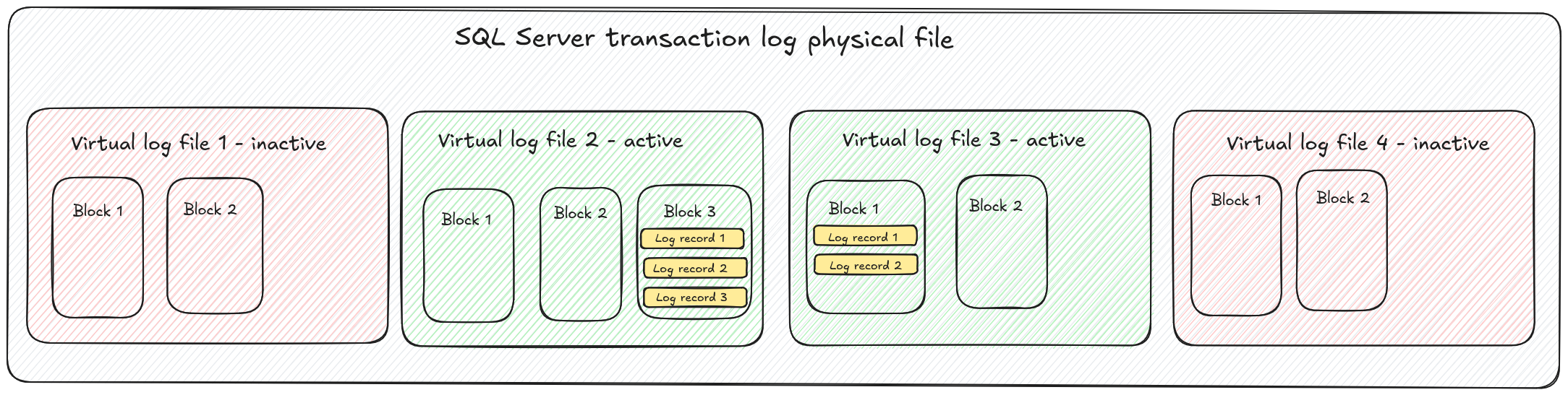
Blocks as well as records in the blocks have assigned unique sequence numbers. Block sequence number is 4 bytes long, while record sequence number is only 2 bytes long. When we put it together with a VLF sequence number, each record can be uniquely identified by triple numbers:
<VLF sequence number>:<block sequence number>:<record sequence number>This unique record identifier is known as log sequence number, usually shortcutted as LSN. This is the number which Debezium uses for storing offsets - what is the latest change seen by Debezium and what is the latest committed transaction processed by Debezium.
SQL Server Data Structure
In the previous chapter, we examined the structure of the SQL Server transaction log. As mentioned earlier, the transaction log records all operations executed against a database. However, since the log can eventually be truncated, the information it contains may be lost. To ensure durability and performance, the actual data and associated metadata (such as indexes) are stored permanently on disk. Let’s take a closer look at how SQL Server organizes this data.
Partitions and Allocation Units
Each table or index is stored in one or more partitions. The maximum number of partitions each table or index can have is 15,000. The subset of the table or index stored in a single partition is called hobt, which is a shortcut from Heap or B-tree. Heap is called a table without clustered index, which data is not organized according to the index. For tables with clustered index, table data is organized according to the index and is actually index rows.
A partition contains the data pages where the actual rows live. There are three main types of data pages. In-row data pages, which store fixed-size data or data which fits into one page. Row-overflow data pages store variable-length data types such as varchar or nvarchar when they don’t fit entirely in-row. LOB data pages store large objects (LOBs), such as xml or large binary data. Pages of the same type within a partition are grouped into allocation units.
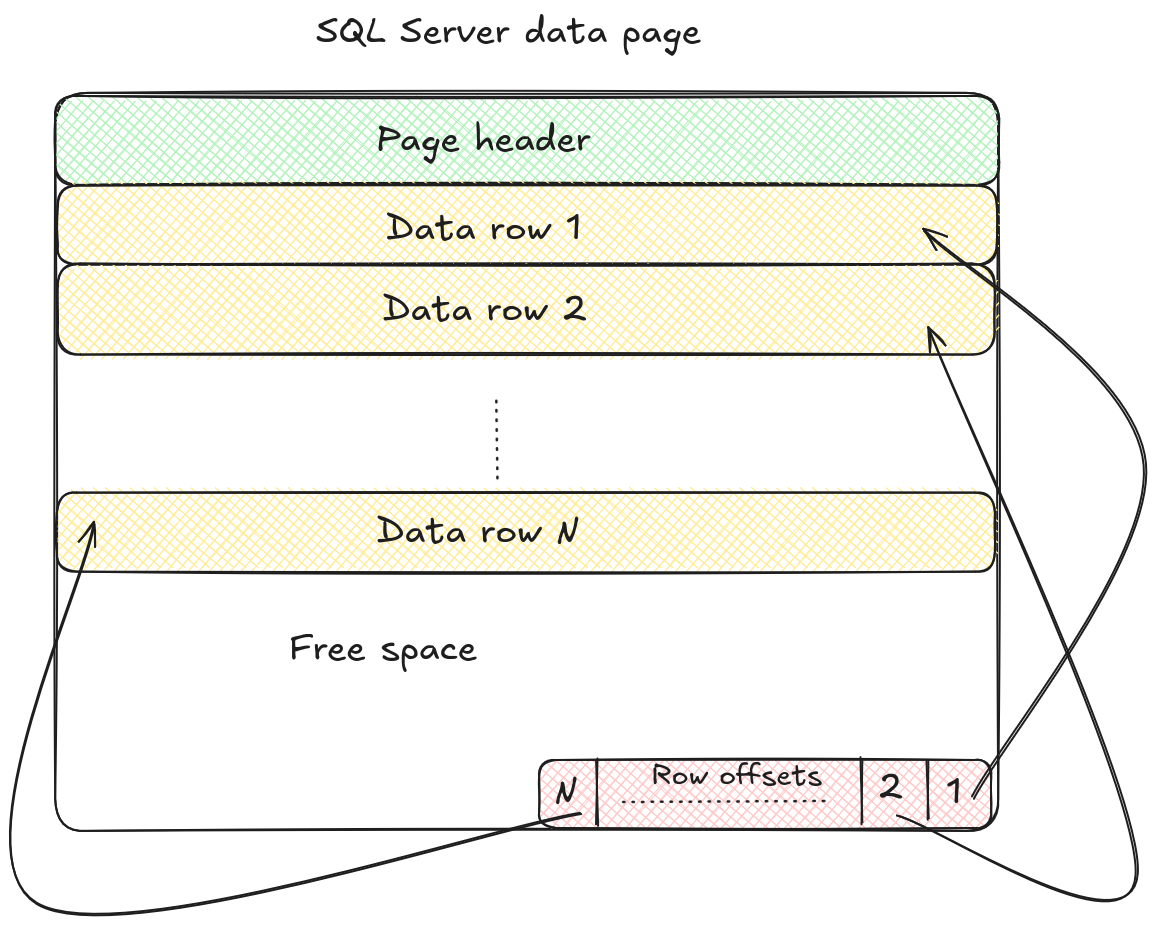
Pages: The Basic Storage Unit
Pages are elementary storage unit in SQL Server and are stored in the .mdf files we discussed earlier. Each .mdf file is divided into 8 KB chunks, and each chunk is what we call a page. A page begins with a 96-byte header, which stores metadata such as page number, page type, amount of free space remaining in the page, number of the allocation unit which owns the page etc. After the header, the data rows are stored. The location of each row within the page is determined by a row offset. A row offset is a two-byte value that indicates how many bytes from the start of the page the row begins at. Offsets are stored in reverse order at the end of the page, forming what’s often called a row offset array. This design makes it easy for SQL Server to find, insert, or move rows within a page without rewriting the entire page. The structure of the page is depicted on the following figure:
Variable-length and LOB objects often cannot fit into a single page, and since rows cannot span multiple pages, these large values are stored outside the in-row data allocation unit. Instead, they are placed in pages managed by either row-overflow or LOB allocation units.
Pages themselves are grouped into so-called extents, which are the basic units SQL Server uses to manage disk space. Each extent consists of 8 pages, covering a total of 64 KB. Extents can be of two types. Uniform extents where all 8 pages belong to the same object and mixed extents where the pages may belong to different objects. SQL Server tracks extent usage with special allocation maps. The Global Allocation Map (GAM) records whether an extent is free or allocated. The Shared Global Allocation Map (SGAM) identifies mixed extents that still contain free pages.
A deeper discussion of these mechanisms is beyond the scope of this blog post, but you can explore more details in the official Pages and Extents Architecture Guide.
Investigating Table and Page Structure
From a practical standpoint, information about indexes, tables, and columns can be queried through the system views sys.indexes, sys.tables, and sys.columns. Details about partitions and allocation units are available in sys.partitions, sys.allocation_units, and eventually also in sys.system_internals_allocation_units. These views can be linked together using the function OBJECT_ID. For example, to determine how many partitions our products table consists of, we can run the following query:
SELECT object_id, partition_id, partition_number, hobt_id
FROM sys.partitions
WHERE object_id = OBJECT_ID(N'products');
The output can look like this:
object_id   partition_id         partition_number hobt_id
----------- -------------------- ---------------- --------------------
  901578250    72057594045726720                1    72057594045726720
The resulting partition_id can then be used to obtain information about allocations for this table:
SELECT *
FROM sys.allocation_units
WHERE container_id = (
    SELECT partition_id
    FROM sys.partitions
    WHERE object_id = OBJECT_ID(N'products')
);
The query gave us following result:
allocation_unit_id   type type_desc                                                    container_id         data_space_id total_pages          used_pages           data_pages
-------------------- ---- ------------------------------------------------------------ -------------------- ------------- -------------------- -------------------- --------------------
   72057594052476928    1 IN_ROW_DATA                                                     72057594045726720             1                    9                    2                    1
By interconnecting these system views, we can gather detailed information about how tables and indexes are structured. However, the views stop short of exposing the actual page contents where data is stored.
Exploring Pages with DBCC IND
To inspect the structure and content of individual pages, SQL Server provides the DBCC utility. Many of the functions we need are undocumented but well described in community resources.
The first useful command is DBCC IND, which returns page information for a given table. The syntax of the command is as follows:
DBCC IND ( [ database_name | database_id ], table_name, index_id )index_id can be taken from sys.indexes, or -1 shows all indexes and IAMs (Index Allocation Maps) and -2 shows only IAMs.
For our products table:
DBCC IND ('TestDB', 'products', -1)results into
PageFID PagePID     IAMFID IAMPID      ObjectID    IndexID     PartitionNumber PartitionID          iam_chain_type       PageType IndexLevel NextPageFID NextPagePID PrevPageFID PrevPagePID
------- ----------- ------ ----------- ----------- ----------- --------------- -------------------- -------------------- -------- ---------- ----------- ----------- ----------- -----------
      1         231   NULL        NULL   901578250           1               1    72057594045726720 In-row data                10       NULL           0           0           0           0
      1         336      1         231   901578250           1               1    72057594045726720 In-row data                 1          0           0           0           0           0
The first record represents the IAM page, while the second corresponds to the actual data page containing table rows. The key values here are PageFID and PagePID, which we’ll use in the next command: DBCC PAGE.
Reading Pages with DBCC PAGE
Another undocumented function of DBCC utility is DBCC PAGE, which dumps the content of the requested page. Before running DBCC PAGE, you must enable trace flag 3604 to send the output to the client:
DBCC TRACEON(3604);The syntax of DBCC PAGE command is
DBCC PAGE ( [ database_name | database_id ], file_number, page_number, print_option )where file_number and page_number are the PageFID and PagePID from DBCC IND. print_option controls detail level and can have values 0–3. Adding WITH TABLERESULTS formats the output in tabular form.
For our data page table:
DBCC PAGE ('TestDB', 1, 336, 0)we get
PAGE: (1:336)


BUFFER:


BUF @0x00000009000FDA40


bpage = 0x000000101A8B0000          bPmmpage = 0x0000000000000000       bsort_r_nextbP = 0x0000000000000000

bsort_r_prevbP = 0x0000000000000000 bhash = 0x0000000000000000          bpageno = (1:336)

bpart = 4                           bstat = 0x10b                       breferences = 0

berrcode = 0                        bUse1 = 22094                       bstat2 = 0x0

blog = 0x1cc                        bsampleCount = 0                    bIoCount = 0

resPoolId = 0                       bcputicks = 0                       bReadMicroSec = 294

bDirtyPendingCount = 0              bDirtyContext = 0x000000100C4947A0  bDbPageBroker = 0x0000000000000000

bdbid = 5                           bpru = 0x00000010047A0040


PAGE HEADER:


Page @0x000000101A8B0000


m_pageId = (1:336)                  m_headerVersion = 1                 m_type = 1

m_typeFlagBits = 0x0                m_level = 0                         m_flagBits = 0x8000

m_objId (AllocUnitId.idObj) = 222   m_indexId (AllocUnitId.idInd) = 256 Metadata: AllocUnitId = 72057594052476928

Metadata: PartitionId = 72057594045726720                                Metadata: IndexId = 1

Metadata: ObjectId = 901578250      m_prevPage = (0:0)                  m_nextPage = (0:0)

pminlen = 16                        m_slotCnt = 3                       m_freeCnt = 7761

m_freeData = 425                    m_reservedCnt = 0                   m_lsn = (42:208:29)

m_xactReserved = 0                  m_xdesId = (0:0)                    m_ghostRecCnt = 0

m_tornBits = 0                      DB Frag ID = 1


Allocation Status


GAM (1:2) = ALLOCATED               SGAM (1:3) = NOT ALLOCATED          PFS (1:1) = 0x40 ALLOCATED   0_PCT_FULL

DIFF (1:6) = CHANGED                ML (1:7) = NOT MIN_LOGGED
The Page Header section reveals useful metadata such as:
-
m_lsn- the log sequence number of the last change to this page, which is useful during recovery process -
m_slotCnt- number of rows (slots) on the page -
pminlen- size of fixed-length data -
m_freeData- offset where free space begins -
m_prevPage/m_nextPage- pointers to neighboring pages (empty here, since we have too little data to span multiple pages)
With print_option set to 1 or 3, DBCC PAGE also shows the byte representation of row contents in the DATA section. You can easily identify variable string column there. For brevity only the first row is shown here:
Slot 0, Offset 0x60, Length 81, DumpStyle BYTE


Record Type = PRIMARY_RECORD        Record Attributes =  NULL_BITMAP VARIABLE_COLUMNS

Record Size = 81
Memory Dump @0x000000096A026060


0000000000000000:   30001000 01000000 1f85eb51 b81e0940 04000002  0........ëQ¸. @....

0000000000000014:   00270051 00730063 006f006f 00740065 00720053  .'.Q.s.c.o.o.t.e.r.S

0000000000000028:   006d0061 006c006c 00200032 002d0077 00680065  .m.a.l.l. .2.-.w.h.e

000000000000003C:   0065006c 00200073 0063006f 006f0074 00650072  .e.l. .s.c.o.o.t.e.r

0000000000000050:   00
At the end of the output you can also see the offset map, dumped at the same (reverse) order, as written on the disk:
OFFSET TABLE:


Row - Offset

2 (0x2) - 254 (0xfe)

1 (0x1) - 177 (0xb1)

0 (0x0) - 96 (0x60)
Conclusion
In this blog post, we explored the basic structure of the SQL Server transaction log and examined how tables are physically stored on disk. The theory was complemented by practical examples - from installing SQL Server to dumping the contents of a data page.
These insights provide a solid foundation for the next post, where we explore ways to parse the SQL Server transaction log programmatically.
About Debezium
Debezium is an open source distributed platform that turns your existing databases into event streams, so applications can see and respond almost instantly to each committed row-level change in the databases. Debezium is built on top of Kafka and provides Kafka Connect compatible connectors that monitor specific database management systems. Debezium records the history of data changes in Kafka logs, so your application can be stopped and restarted at any time and can easily consume all of the events it missed while it was not running, ensuring that all events are processed correctly and completely. Debezium is open source under the Apache License, Version 2.0.
Get involved
We hope you find Debezium interesting and useful, and want to give it a try. Follow us on Twitter @debezium, chat with us on Zulip, or join our mailing list to talk with the community. All of the code is open source on GitHub, so build the code locally and help us improve ours existing connectors and add even more connectors. If you find problems or have ideas how we can improve Debezium, please let us know or log an issue.